Neural networks, an important tool for processing data in a variety of industries, grew from an academic research area to a cornerstone of industry over the last few years. Convolutional Neural Networks (CNNs) have been particularly useful for extracting information from images, whether classifying them, recognizing faces, or evaluating board positions in Go.
At Uber, we use CNNs for an assortment of purposes, from detecting objects and predicting their motion to processing petabytes of street-level and satellite images to improve our maps. When making use of a CNN, we care about how accurately it completes its task, and in many cases, we also care about its speed. In these two examples, a network twice as fast may enable real-time detection instead of offline detection or be able to process an enormous dataset in one week of data center time instead of two.
In this article, we describe an approach presented at NeurIPS 2018 for making CNNs smaller, faster, and more accurate all at the same time by hacking libjpeg and leveraging the internal image representations already used by JPEG, the popular image format. An earlier version of this work was presented as an ICLR workshop poster in June 2018. This article will also discuss surprising insights about frequency space and color information as they relate to network architecture design.
To understand the approach, first let’s look at how the JPEG codec works. Once we understand JPEG, how we may apply a CNN will follow naturally.
How JPEG works
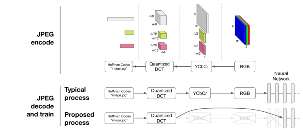
JPEG is an old format, having celebrated its 25th birthday in 2017, and remains one of the most widely used image formats. In one of its common configurations, the JPEG encoder proceeds through the steps in Figure 1, below, shown right-to-left:
Starting with an RGB representation of an image (shown on the right), the image is converted to the YCbCr color space—Y representing luminance (brightness) and the Cb and Cr channels representing the chroma (hue). The Cb and Cr channels are then downsampled by a predetermined factor, usually two or three (in our work, we use a factor of two). This downsampling is the first stage of compression: the first stage at which information is lost. Each channel in this representation is then split into 8×8 blocks and put through the discrete cosine transform (DCT), a transform to frequency space similar to a Fourier transform. The DCT itself is lossless and reversible, transforming an 8×8 spatial block into 64 channels.
The coefficients are then quantized, a process which is lossy and comprises the second compression stage. Quantization is controlled by the JPEG quality parameter, with lower quality settings corresponding to more severe compression and resulting in smaller files. Quantization thresholds are specific to each spatial frequency and have been carefully designed: less compression is applied to low frequencies than high frequencies, as the human eye is more sensitive to subtle errors over broad areas than changes in magnitude of high frequency signals. The quantized DCT coefficients (integers) are then compressed losslessly by a variant of the Huffman encoding and stored in a JPEG file, like the image.jpg shown in Figure 1, above.
The JPEG decoding process is simply the reverse of the JPEG encoding process. All reversible steps are inverted exactly, and the two lossy steps—quantization and downsampling—are approximately inverted to produce an RGB image. For context, this process has probably been run ten times just to decode and display the images shown on this web page!
Let’s say we’d like to train a neural network on a JPEG image. We can decompress the JPEG image to RGB and feed it into the first layer of a neural network, as depicted in Figure 2, below:

Now that we understand the JPEG algorithm, can’t we easily do better? There’s no reason neural nets have to process images represented as an array of RGB pixels. And many neural nets seem to learn a transformation from pixel space to frequency space in their first layers. So, as depicted in Figure 3, below, why not just feed the DCT representation directly into the network, skipping some early layers in the process?

This is exactly the approach we detail below and in our paper: we modify libjpeg to output DCT coefficients directly to TensorFlow (our code is available if you want to try for yourself) and train networks directly on this representation. It turns out to work really well as long as one gets a few details right!
Baselines
In our research, we trained networks from a JPEG representation, hoping for the resulting networks to be both accurate and fast to execute. There were several image processing tasks we considered, but for now we chose to experiment on classifying images from the ImageNet dataset. All networks we used were based on the Residual Network ResNet-50, and all were trained for 90 epochs, which can be accomplished in our set-up in only two to three hours by using Horovod to take advantage of distributed training across 128 NVIDIA Pascal GPUs.
First, we trained a vanilla ResNet-50 in the most standard way—from RGB pixels—and found that it attains a top-five error of about 7.4 percent and could run inference on just over 200 images per second on an NVIDIA Pascal GPU. In Figure 4, below, we depict that network as a small black square on a plot that traces the relationship between error rate and speed:
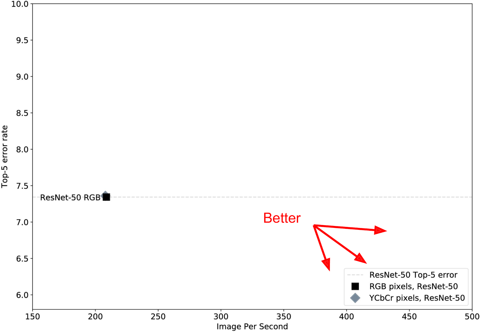
The gray dotted line shows this baseline level of accuracy. We prefer networks that are faster to ones that are slower and networks that have lower error to ones with higher error, so we wanted to find networks that appear down and to the right in this plot. Depending on the specific application, we might be willing to make tradeoffs in terms of accuracy and speed. In addition to the RGB pixel network, we also trained a network from YCbCr pixels (gray diamond under the square) and found it to perform just about identically, showing that color space on its own doesn’t significantly affect performance here.
Since we aimed for networks that are fast and accurate, we first tried making ResNet-50 shorter (removing blocks from the bottom) or thinner (using fewer channels per layer). While this makes the networks faster, how much accuracy will we lose? In Figure 5, below, a few shorter and thinner networks display the trade-off curve available to us by simple mutations of ResNet-50 that still leverage RGB pixel input:
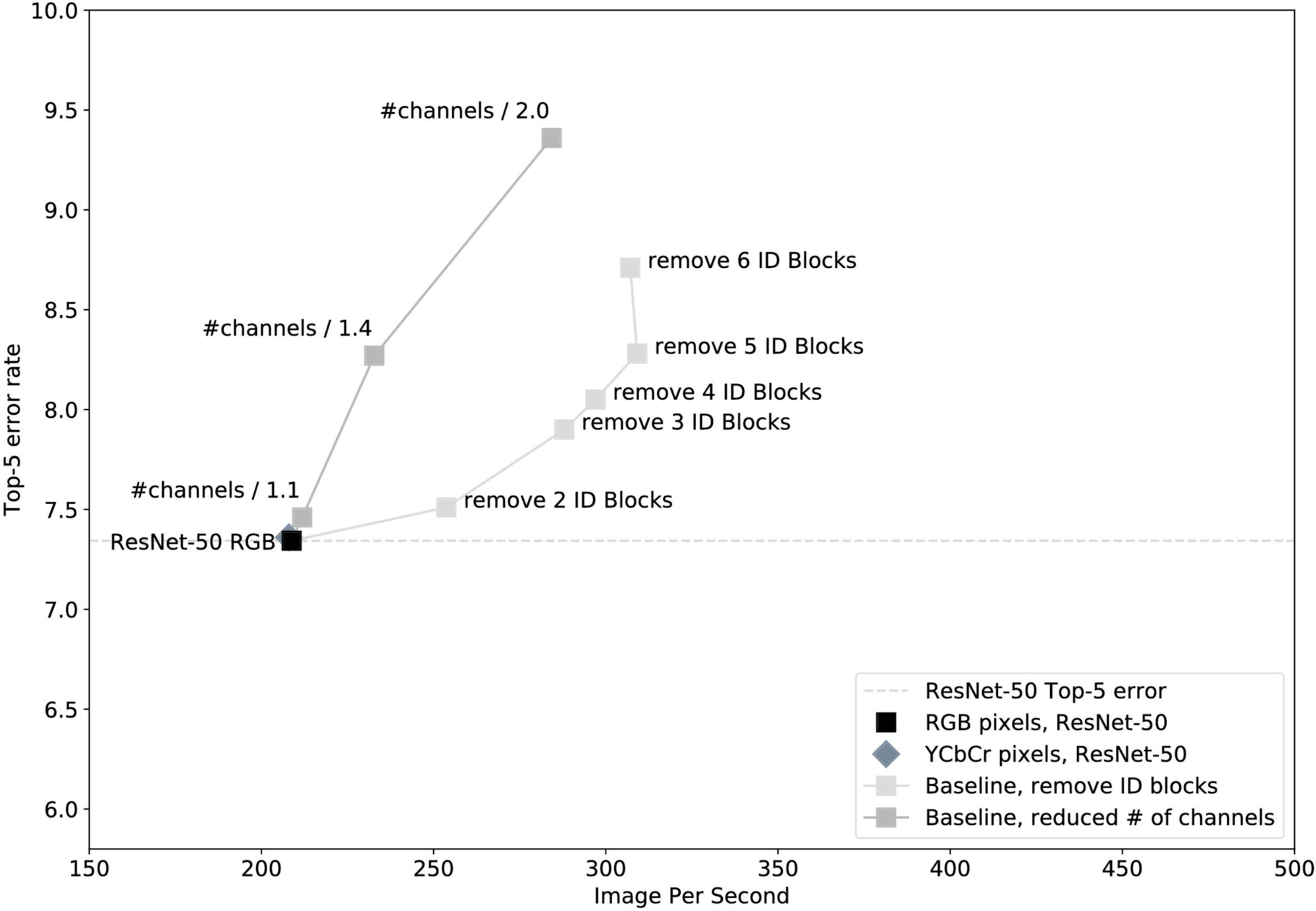
In Figure 5, we can see that shorter networks with full width fare better than thin networks that maintain full depth. The light gray “Remove N ID Blocks” line forms the Pareto front, showing the set of “non-dominated” networks, or those networks offering the best possible speed vs. accuracy tradeoffs. For example, simply removing three ID blocks gives us a boost to almost 300 images per second, but errors also increase, in this case to nearly eight percent. The “Remove 3 ID Blocks” network is on the Pareto front because no other network has both lower error and higher speed than it. (More details about these networks are available in our full research paper.)
Now let’s try training networks directly on the DCT coefficients available in the JPEG decoder to see if we can push the whole Pareto front forward.
Training networks on DCT inputs
To train from DCT input, we must first consider the problem of different input sizes.
The vanilla ResNet-50 is designed for inputs with shape (224, 224, 3) — width and height of 224 pixels and 3 color channels (RGB). Our DCT coefficients are very differently shaped: the Y channel is 8x smaller along each spatial dimension but has 64 frequency channels, resulting in input shape (28, 28, 64). The Cb and Cr channels are 16x smaller (due to the additional 2x downsampling), so they each have shape (14, 14, 64). How should we deal with representations of these unusual shapes?
Assuming we do not completely ignore either input, a basic requirement of any proposed architecture is that it eventually combines Y and Cb/Cr before making a classification decision. All architectures we will consider are of the following form: apply a transform or sub-network T1 to Y, apply another transform or sub-network T2 to Cb and Cr, concatenate the results channel-wise, and feed the concatenated representation to a ResNet mirroring the top of ResNet-50 with or without some modifications. The general architecture is depicted in Figure 6, below:
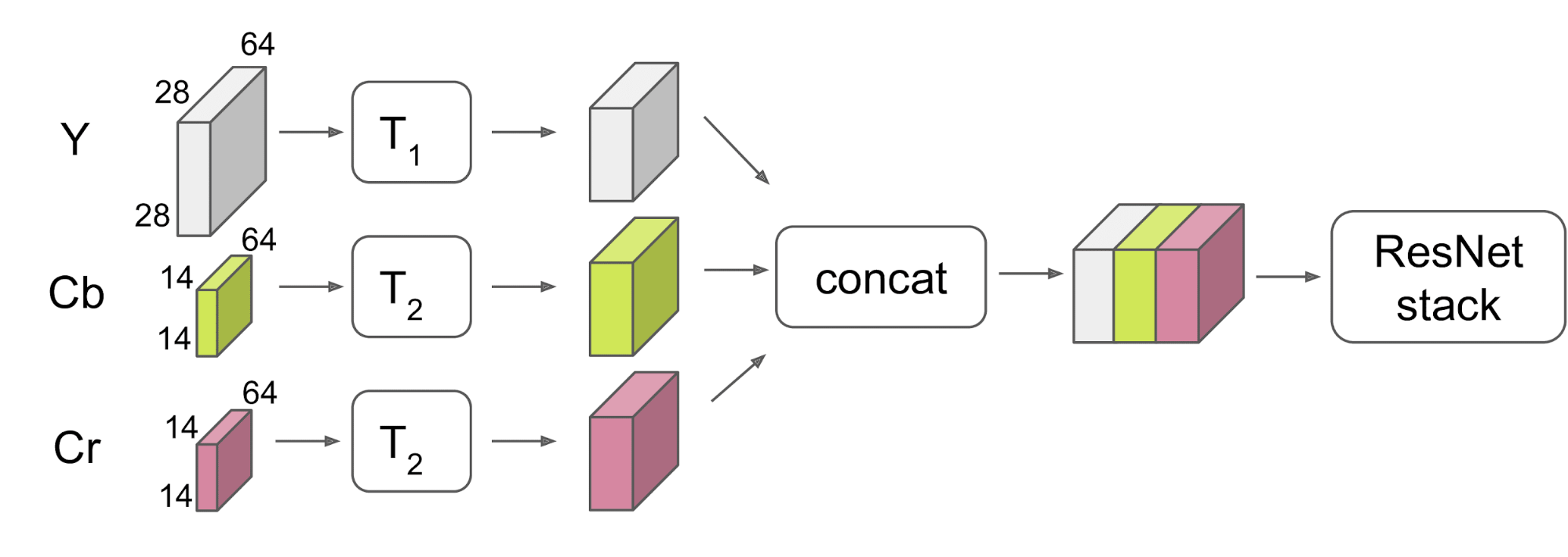
In cases where T2 is a sub-network (learned transform), the weights are unshared between the Cb and Cr paths. Note that in order to concatenate the representations channel-wise, they must share the same spatial size, so, for example, it is not possible for T1 and T2 both to be identity transforms.
We consider two families of T1 and T2 transforms: those that merge paths early by using at most single-layer transforms, and those that do more significant processing first, merging paths late.
DCT Early Merge architectures
The simplest way of making the disparate spatial sizes of Y and Cb/Cr match is to downsample the large representation (Y) or upsample the small representations (Cb/Cr). We try both and add the results to our plot as blue “DownSampling” and “UpSampling” circles, depicted in Figure 7, below:

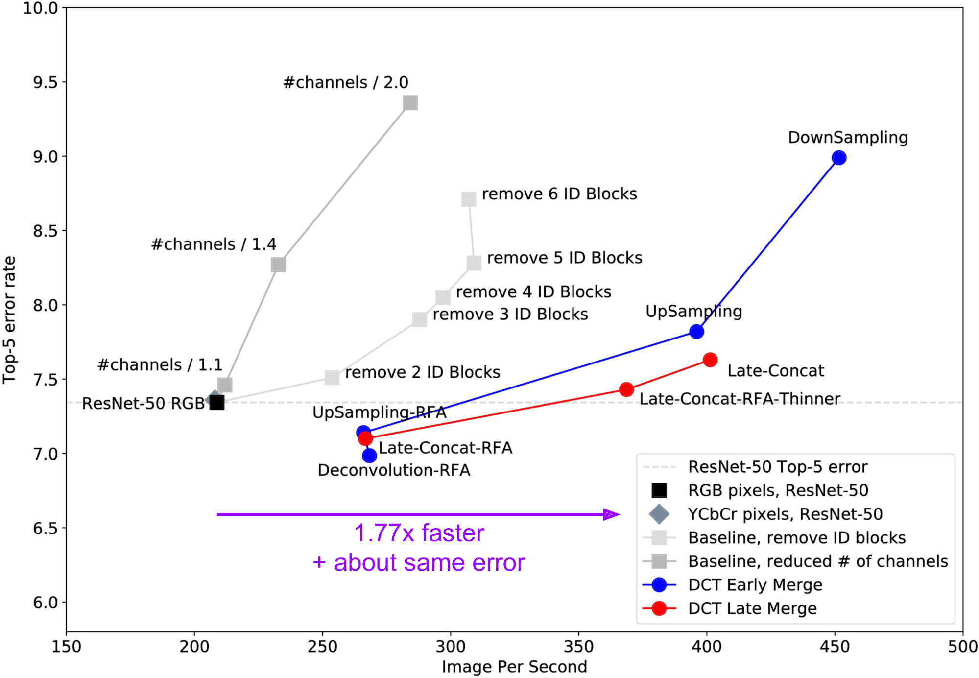
Because the DownSampling model reduces the spatial size of input data at the first layer, it ends up being very fast—about 450 images per second, or more than twice the speed of ResNet-50—but its error is also much higher. The UpSampling model is slower and more accurate because it throws away less information.
We were initially a little disappointed that the error in the UpSampling model was higher than the baseline ResNet-50. We hypothesized that the source of this problem was a subtle issue: units in early layers in the DownSampling and UpSampling models have receptive fields that are too large. The receptive field of a unit in a CNN is the number of input pixels that it can see, or the number of input pixels that can possibly influence its activation. Indeed, after examining the strides and receptive fields of each layer in the network, we found that halfway through a vanilla ResNet-50, units have receptive fields of about 70. Just as far through our naively assembled UpSampling model the receptive fields are already 110px, larger because our DCT input layer has [stride, receptive field] of [8, 8] instead of the typical typical [1, 1] pixel input layer. Intuitively we’re asking the network to learn about 110px wide visual concepts but not giving it enough layers or computational capacity to do so. (See Section 3 and Figure 4 in our full paper for more discussion.)
We created a new Receptive Field Aware (RFA) model, UpSampling-RFA, by adding extra stride-1 blocks early in the network. With this new model, the growth of receptive field layer-by-layer is now smoother, approximately matching that in ResNet-50, and performance is increased (see Figure 7). If the upsampling is done via learned Deconvolution instead of pixel duplication, error is further reduced, producing the best model yet: Deconvolution-RFA.
By being careful about receptive fields, we’ve now discovered a model that is both more accurate (6.98 percent compared to 7.35 percent error) and 1.29x faster than the baseline! Other models along the same DCT Early Merge line now form the new Pareto front, dominating previous models in terms of the error and speed trade-offs they offer.
Next, we try deeper learned T1and T2 transforms to see if we can push the frontier further.
DCT Late Merge architectures
Merging the Y and Cb/Cr channels early follows the typical and conceptually simple deep learning paradigm: get all the data together somehow, give it to the model, and let the model learn what to do with it. This approach is elegant in its simplicity, but could we produce even faster models by eliminating unneeded computation?
After some experimentation, we found that allowing the luminance branch many layers of computation was required for high accuracy, but the chroma paths could be afforded fewer layers of computation without detriment. In other words, putting the Y channel into the bottom of the network and then injecting Cb/Cr information halfway through works just as well as starting with all three at the bottom, but, of course, the former saves computation.
As depicted in Figure 8, below, we show the resulting speed and error rate of this Late-Concat model in red, together with two related networks: a receptive field aware version, Late-Concat-RFA, and a version tweaked for speed by using fewer filters, Late-Concat-RFA-Thinner. As we can see, the Pareto front moves forward once again! In particular, we now have found a model 1.77x faster than a vanilla ResNet and with nearly the same rate of error.
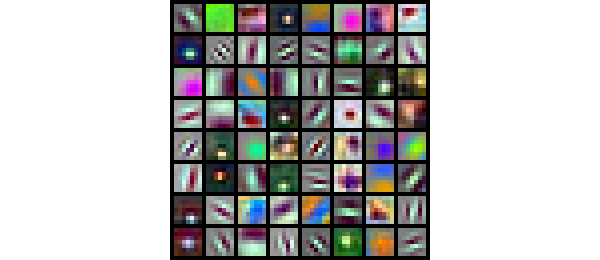
It is interesting that color information is not needed until later in the network, when it is combined with higher-level concepts learned from luminance. At this point we can only speculate, but it may be that learning mid-level concepts (for example: grass or dog fur) requires several layers of processing fine brightness edges into textures before being combined with spatially less precise color information (for example: green or brown). Perhaps we could have expected this result (Figure 9) all along from the higher frequency black and white edges and lower frequency (or constant) color detectors learned by ResNet-50 from RGB pixels.
Pinpointing gains and future directions
The results we’ve shown so far are encouraging and useful to practitioners—we’ve shown what works to produce fast and accurate networks. To make this contribution to the field meaningful scientifically, we also need to pinpoint these gains and show why they are realized. In our paper, we perform ablation studies to identify sources of gains.
In summary, we found that speed gains are simply due to a smaller volume of data on the input layer and subsequent layers, as one might expect. Accuracy gains are due primarily to the specific use of a DCT representation, which turns out to work curiously well for image classification. Surprisingly, simply replacing the first convolutional layer of a ResNet-50 with the stride 8 DCT transform results in much better performance. It works even better than a learned transform of exactly the same shape. In other words, in contrast to conventional wisdom, we find that using larger receptive fields and strides (of 8 each) works better than small, and hard coding the first layer works better than learning it. When Residual Networks set the state of the art on ImageNet in 2015, simply replacing the first layer with a frozen DCT would have further improved the state of the art.
Future directions suggested by the above results include evaluating different frequency space representations, DCTs of different sizes, and performance on detection, segmentation, and other image-processing tasks.
If you work on any image processing using neural networks, we’d love to hear if switching to a DCT representation benefits your task as well as it has here. If you’d like a more detailed description of these results, see our paper (including architectural details in the Supplementary Information section) and make use of our codebase to easily read DCT representations into TensorFlow or PyTorch.
If this type of research interests you, consider applying for a role at Uber AI Labs.

Lionel Gueguen
Lionel Gueguen is a senior software engineer with Uber ATG.

Rosanne Liu
Rosanne is a senior research scientist and a founding member of Uber AI. She obtained her PhD in Computer Science at Northwestern University, where she used neural networks to help discover novel materials. She is currently working on the multiple fronts where machine learning and neural networks are mysterious. She attempts to write in her spare time.

Alex Sergeev
Alex Sergeev is a deep learning engineer on the Machine Learning Platform team.
Jason Yosinski
Jason Yosinski is a former founding member of Uber AI Labs and formerly lead the Deep Collective research group.
Posted by Lionel Gueguen, Rosanne Liu, Alex Sergeev, Jason Yosinski
Related articles
Most popular
Migrating a Trillion Entries of Uber’s Ledger Data from DynamoDB to LedgerStore

Ensuring Precision and Integrity: A Deep Dive into Uber’s Accounting Data Testing Strategies

DragonCrawl: Generative AI for High-Quality Mobile Testing

DataCentral: Uber’s Big Data Observability and Chargeback Platform
Products
Company

